From classical to quantum: bits to qubits#
Author: Alexandra Semposki
Maintainer: Alexandra Semposki
What is the first thing that a person beginning their journey in quantum computing needs to understand? Well, this could be a rather contested statement, but arguably the most important bit of information (pun intended) is the qubit. What is a qubit? How does this tie into the classical computing we’re all used to? How does a qubit rely on quantum mechanics and how can we get information from one? All of these questions will be answered shortly in this section, so read on!
What are qubits?#
Jumping right into it, a qubit is the quantum mechanical equivalent of a classical bit, which you saw in any computer science or computational physics course. What was the bit defined as then? A bit is a small amount of information stored in a computer using binary code, i.e. 0 or 1. When it comes down to it, all information is stored in this way, with strings of 0s and 1s building up to more and more complex pieces of data.
With this concept established, a qubit is then a piece of information stored in a quantum mechanical way, instead of a classical way. They are still like bits, in that they store small snippets of information and can be built up into larger and larger data sources, but they differ in this quantum mechanical sense from their classical counterparts, which we will see below.
Qubit representation#
In classical cases, you will see the bit simply represented as 0 or 1, as just discussed above. However, this changes when one is looking at a qubit. Qubits can be represented using Dirac notation—from elementary quantum mechanics—as
which qualify as a qubit state. This can be better written as
But wait! What is this? Qubit states can be written as a superposition of individual qubits? This is where the quantum mechanical effect starts to rear its head. \(| \psi \rangle\) above is absolutely in a superposition of the states \(|0\rangle\) and \(|1\rangle\), and this gives rise to two very important points:
A qubit state does not have to be only in the state 0 or 1 (though it can be in only one of those two states); it can also be in any superposition of the two, leading to an infinite number of possible qubit states. This is in stark contrast to the classical bit, which has only the two possible states of 0 and 1.
Probability must now be not only considered, but also conserved, which means taking care to keep track of the coefficients \(\alpha\) and \(\beta\) in \(| \psi \rangle\) above. After all, quantum mechanics is highly probabilistic, and this will come up again and again in quantum computing.
From the second point above, these states follow the rule that, in order to conserve probability (and hence normalize the statevector)
This also helps lend credence to the first point above—\(\alpha\) and \(\beta\) could be any two numbers that sum to one. We’ll get into their significance in the Measurement of qubits section below.
Converting the coefficients#
Before we talk about measuring or visualizing the qubit state, we want to think about the coefficients of the two states \(|0\rangle\) and \(|1\rangle\) as real numbers. To avoid them being complex, we can first pull any complex numbers out of the coefficients by writing
where the \(\phi\) angle is now considered the phase of the qubit state. We could, of course, have written an global phase for the entire statevector \(|\psi\rangle\), but this would not be a phase we could measure—how would one measure something when one has no reference point to consider? Hence we do not write any overall phase factor, only the one contained in \(e^{i\phi}\). This form of the statevector will also help tremendously in making sure we know which state we are considering [2]. Why is the phase here attached to only one of the individual states? Because it is the relative phase between the \(|0\rangle\) state and the \(|1\rangle\) state [2].
We can continue on to define the coefficients in a trigonometric fashion instead of just \(\alpha\) and \(\beta\)—this can be done by writing the statevector \(|\psi\rangle\) as
where \(\theta\) is now contained in the coefficients of both states. These actions have changed our unknown variables from \(\alpha\) and \(\beta\) to \(\theta\) and \(\phi\), and this will now make it much easier to visualize the qubit statevector.
Visualizing a qubit state#
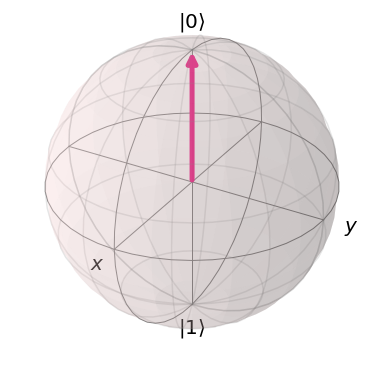
A qubit state can be thought of as a vector in a portion of Hilbert space that can be seen on a sphere if we consider the coordinates to be spherical (with \(r\), the magnitude of the statevector, set to 1) [2]. With \(\theta\) and \(\phi\) now understood, we can finally take a look at an example of a qubit statevector with \(\theta = 0\) and \(\phi = 0\). This means our statevector now looks like
Below we can use Qiskit, the IBM Quantum Computing package, to visualize the vector on the Bloch sphere.
#import Qiskit package
from qiskit import visualization

#plot the Bloch sphere with selected vector (in cartesian coordinates!)
visualization.plot_bloch_vector([0,0,1])
Measurement of qubits#
Measuring qubits will be covered in more detail later on when we actually look at how circuits can be built with multiple qubits included, but for now we will talk a little bit about how to measure one. Recalling what we know from quantum mechanics, measuring the state of a system will collapse the wavefunction of that state into a definite answer that will no longer be fluid, or a superposition of states. This same principle applies in quantum computing to qubits: if the qubit’s state is measured, it will collapse into either the \(|0\rangle\) state or the \(|1\rangle\) state. No matter how many times it is measured, no other measurement outcome will be seen. How, then, can we know what the probability is for obtaining either 0 or 1 as a result?
As in statistical mechanics, an ensemble of identical states must be ‘’prepared’’ to tackle this problem. If we measure each individual state in the ensemble, and they are all identical, their measurements will give us an idea of this probability as more and more measurements are made.
Later on, when we do actual measurements on either a simulator or an actual quantum computer, we will see that a number of shots must be made when making these measurements on qubit states, and usually this is a very large number (such as \(2^{13}\) shots). This is so we have enough identically prepared states to gain a concrete estimate of the probability of our measuring either 0 or 1 from our qubit. And what does this probability correspond to? Of course, the coefficient of our \(|0\rangle\) and \(|1\rangle\) states in our overall statevector!
In the next section, we will take a look at quantum gates and how to use qubits with these gates in simple quantum circuits.
References#
[1] Nielsen, M. A., & Chuang, I. L. (2011). Quantum Computation and Quantum Information: 10th Anniversary Edition. Cambridge University Press.
[2] Qiskit textbook, “Quantum States and Qubits: Representing Qubit States” (exact page found here).